Understand the data¶

Import the data ¶

Before anything else, we will take a look at the data we will work with in this section. Let’s start by importing the datasets, using the function read_csv() from the library Pandas. We will use two datasets containing AIS data.

import pandas as pd

dynamic_data = pd.read_csv('./dynamic_data.csv')
static_data = pd.read_csv('./static_data.csv')

The data are imported from the U.S. Marine Cadastre website and are publicly available here: https://marinecadastre.gov/ais/. The datasets used here are a slightly modified version of the raw datasets available on the website, to match the needs of this course. For more information about the modifications done to these datasets, visit this page.

When dealing with any data related problem, the first step is to fully understand the data we are using. This means knowing what the data represent and understand the meaning of each attribute.

In addition, some important points must be known by the scientist using the data for a problem, specifically:

where the data come from: which open organism, company, person, collected the data in the first place.
when the data have been collected: most data can vary over time (for example, the number of passengers using a transportation service will vary over the years in an expanding city).
the range of the data: for example, for geographical data, the area of collection has to be known.
how the data have been acquired: the data might have been recorded with sensors or hand tools, collected by person through forms, automatically created with a software, …
if the data have been previously modified: the organism that collected the data in the first place might have done a work of preprocessing before handing them over to further partners.

AIS data in general ¶

Most navigating vessel today in the world must be equiped with an AIS (Automatic Identification System) transponder which sends information about the ships’s status and position at regular intervals of time (every 1 to 3 minutes). The data is collected by coastal stations and other ships, message after message. A message is sent at a certain timestamp by a certain ship, and can contain either static or dynamic information about the ship and the trip it is currently on.

The dynamic information are information that may change every time a new message is sent, such as the speed of the ship, its heading, or its position (latitude and longitude). The static information stay the same for the whole trip of one ship, for example the identification of the ship (MMSI), the destination information, the type of the ship, …

from IPython.display import IFrame
IFrame("https://www.youtube.com/embed/LQyGorGLYGU", "560", "315")

In this part, you have the role of a data scientist in charge of examining and working with AIS data collected from a coastal station next to Seattle (United States). The data you are using have been collected by the U.S. Marine Cadastre on the 1st of January 2017, on the area UTM10 (west coast of the United States and Canada). The exact latitude range is [32.20937 ; 49.89074] and the longitude range is [-125.99859 ; -120.00242], which is comprised in this area:

text

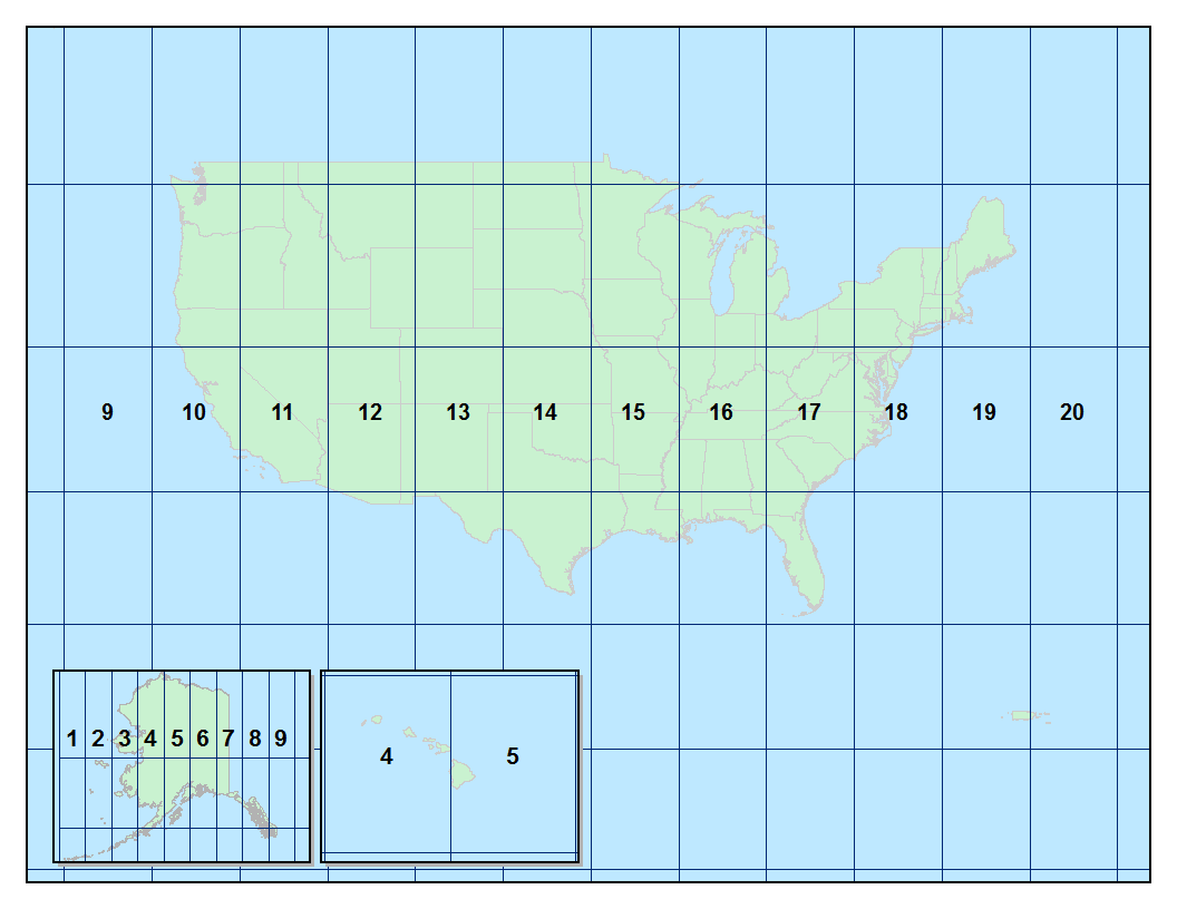
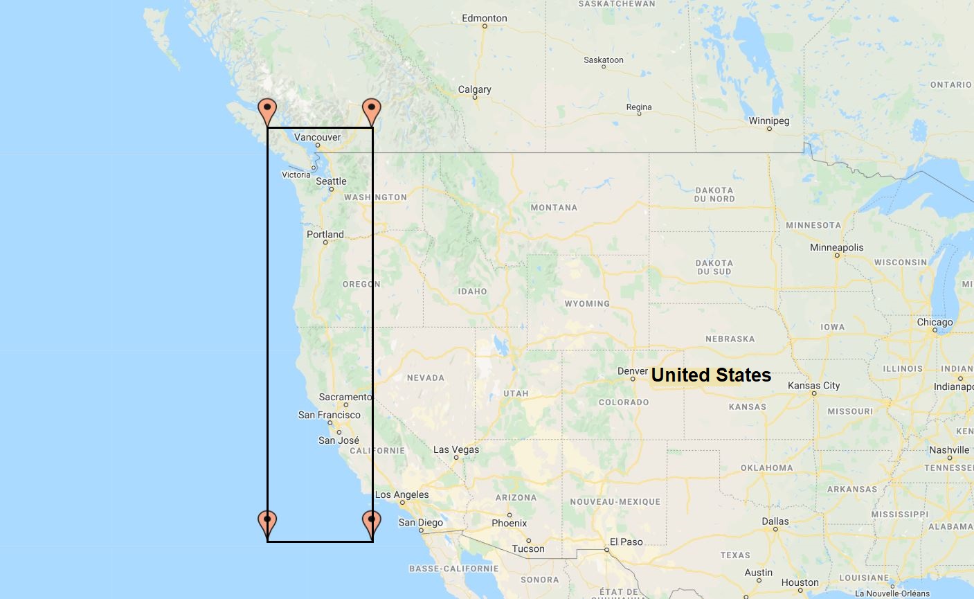
This area, being on the coast, contains several harbours, which makes it interesting for our use.

Dynamic data ¶

We start by printing a part of the dataset, to visualize it. The data you have to work with look like this:

The function head() allows you to print the first elements of a pandas DataFrame.

dynamic_data.head()

	MMSI	BaseDateTime	LAT	LON	SOG	COG	Heading	VesselName	IMO	CallSign	...	DepTime	ArrTime	DepLat	DepLon	ArrLat	ArrLon	DepCountry	DepCity	ArrCountry	ArrCity
0	367114690	2017-01-01 00:00:06	48.51094	-122.60705	0.0	-49.6	511.0	NaN	NaN	NaN	...	2017-01-01 00:00:06	2017-01-01 02:40:45	48.51094	-122.60705	48.51095	-122.60705	US	Anacortes	US	Anacortes
1	367479990	2017-01-01 00:00:03	48.15891	-122.67268	0.1	10.1	353.0	WSF KENNEWICK	IMO9618331	WDF6991	...	2017-01-01 00:00:03	2017-01-01 02:40:44	48.15891	-122.67268	48.11099	-122.75885	US	Coupeville	US	Port Townsend
2	368319000	2017-01-01 00:00:08	43.34576	-124.32142	0.0	32.8	173.0	NaN	NaN	NaN	...	2017-01-01 00:00:08	2017-01-01 02:44:48	43.34576	-124.32142	43.34578	-124.32141	US	Barview	US	Barview
3	367154100	2017-01-01 00:00:15	46.74264	-124.93125	6.8	6.0	352.0	NaN	NaN	NaN	...	2017-01-01 00:00:15	2017-01-01 02:33:28	46.74264	-124.93125	47.02928	-124.95153	US	Ocean Shores	US	Ocean Shores
4	367446870	2017-01-01 00:00:59	48.51320	-122.60718	0.0	23.2	511.0	NaN	NaN	NaN	...	2017-01-01 00:00:59	2017-01-01 02:42:54	48.51320	-122.60718	48.51318	-122.60699	US	Anacortes	US	Anacortes

5 rows × 26 columns

This dataset contains a mix of dynamic and static attributes, as explained earlier. The mention artificially created from original data means that this attribute was added by us to the data downloaded.

Static attributes:

MMSI: unique 9-digit identification code of the ship - numeric
VesselName: name of the ship - string
IMO: unique 7-digit international identification number, that remains unchanged after the transfer of the ship’s registration to another country - numeric
CallSign: unique callsign of the ship - string
VesselType: type of the ship, numerically coded, see here for details - numeric
Length: length of the ship, in meters - numeric
Width: width of the ship, in meters - numeric
Draft: vertical distance between the waterline and the bottom of the hull of the ship, in meters. For one ship, varies with the load of the ship and the density of the water - numeric
TripID: (artificially created from original data) unique ID for the trip - numeric
DepTime: (artificially created from original data) departure time for the trip - datetime
ArrTime: (artificially created from original data) arrival time for the trip - datetime
DepLat: (artificially created from original data) departure latitude for the trip - numeric
DepLon: (artificially created from original data) departure longitude for the trip - numeric
ArrLat: (artificially created from original data) arrival latitude for the trip - numeric
ArrLon: (artificially created from original data) arrival longitude for the trip - numeric
DepCountry: (artificially created from original data) departure country for the trip - string
DepCity: (artificially created from original data) departure city for the trip - string
ArrCountry: (artificially created from original data) arrival country for the trip - string
ArrCity: (artificially created from original data) arrival city for the trip - string

Dynamic attributes:

BaseDateTime: timestamp of the AIS message - datetime
LAT: latitude of the ship (in degree: [-90 ; 90], negative value represents South, 91 indicates ‘not available’) - numeric
LON: longitude of the ship (in degree: [-180 ; 180], negative value represents West, 181 indicates ‘not available’) - numeric
SOG: speed over ground, in knots - numeric
COG: course over ground, direction relative to the absolute North (in degree: [0 ; 359]) - numeric
Heading: heading of the ship (in degree: [0 ; 359], 511 indicates ‘not available’) - numeric
Status: status of the ship - string

from IPython.display import IFrame
IFrame("https://www.youtube.com/embed/3M7mxBimT70", "560", "315")

Static data ¶

From the AIS data collected on the Marine Cadastre Website, we have created a smaller dataset containing only the static data of the trips. This will allow you to compare and analyze the trips as entities. Let’s have a look at these data.

static_data.head()

	TripID	MMSI	MeanSOG	VesselName	IMO	CallSign	VesselType	Length	Width	Draft	...	ArrTime	DepLat	DepLon	ArrLat	ArrLon	DepCountry	DepCity	ArrCountry	ArrCity	Duration
0	1	367114690	0.000000	NaN	NaN	NaN	NaN	NaN	NaN	NaN	...	2017-01-01 02:40:45	48.51094	-122.60705	48.51095	-122.60705	US	Anacortes	US	Anacortes	0 days 02:40:39
1	2	367479990	6.536585	WSF KENNEWICK	IMO9618331	WDF6991	1012.0	83.39	19.5	3.2	...	2017-01-01 02:40:44	48.15891	-122.67268	48.11099	-122.75885	US	Coupeville	US	Port Townsend	0 days 02:40:41
2	3	368319000	0.000758	NaN	NaN	NaN	NaN	NaN	NaN	NaN	...	2017-01-01 02:44:48	43.34576	-124.32142	43.34578	-124.32141	US	Barview	US	Barview	0 days 02:44:40
3	4	367154100	6.871111	NaN	NaN	NaN	NaN	NaN	NaN	NaN	...	2017-01-01 02:33:28	46.74264	-124.93125	47.02928	-124.95153	US	Ocean Shores	US	Ocean Shores	0 days 02:33:13
4	5	367446870	0.000000	NaN	NaN	NaN	NaN	NaN	NaN	NaN	...	2017-01-01 02:42:54	48.51320	-122.60718	48.51318	-122.60699	US	Anacortes	US	Anacortes	0 days 02:41:55

5 rows × 22 columns

As you can see, most of the attributes are the same as for the dynamic data, only the dynamic attributes (like timestamp, latitude, longitude, speed and heading) have disappeared.

Two attributes are new here:

MeanSOG: the mean of the value of the SOG attribute for all the points in the trip - numeric
Duration: the total duration of the tracked trip - numeric

Comparison of dynamic and static datasets ¶

This dataset is built from the same data as the dynamic dataset and therefore contains the same data.

The only difference is that it contains one instance for each trip, instead of one instance for each AIS message.

We can verify that by printing the information of the dataset:

static_data.info()

<class 'pandas.core.frame.DataFrame'>
RangeIndex: 1520 entries, 0 to 1519
Data columns (total 22 columns):
 #   Column      Non-Null Count  Dtype  
---  ------      --------------  -----  
 TripID      1520 non-null   int64  
 MMSI        1520 non-null   int64  
 MeanSOG     1520 non-null   float64
 VesselName  1442 non-null   object 
 IMO         538 non-null    object 
 CallSign    1137 non-null   object 
 VesselType  1287 non-null   float64
 Length      1220 non-null   float64
 Width       911 non-null    float64
 Draft       496 non-null    float64
Cargo       378 non-null    float64
DepTime     1520 non-null   object 
ArrTime     1520 non-null   object 
DepLat      1520 non-null   float64
DepLon      1520 non-null   float64
ArrLat      1520 non-null   float64
ArrLon      1520 non-null   float64
DepCountry  1520 non-null   object 
DepCity     1520 non-null   object 
ArrCountry  1520 non-null   object 
ArrCity     1520 non-null   object 
Duration    1520 non-null   object 
dtypes: float64(10), int64(2), object(10)
memory usage: 261.4+ KB

Where we see that the dataset contains 1520 entries, the number of different trips in the dynamic dataset.

We can verify that by comparing the MMSIs of the ships tracked in both datasets. For that, we collect the unique values of the attribute MMSI in both datasets with the function unique().

We could then print the two lists and visually compare them, but they both contain 1520 values and it would be a long work. Instead, we will check the difference between both by using two loops and printing the elements that are present in one list and not in the other.

We do that two times: diff1 contains the elements present in the dynamic dataset but not in the static one, and diff2 contains the elements present in the static dataset but not in the dynamic one.

# Get the unique MMSI values in both datasets
dynamic_mmsi = dynamic_data['MMSI'].unique()
static_mmsi = static_data['MMSI'].unique()

# Print the two lists
print('dynamic: ' + str(dynamic_mmsi))
print('static: ' + str(static_mmsi))

# Check for elements in dynamic_mmsi that are not in static_mmsi
diff1 = []
for element in dynamic_mmsi:
    if element not in static_mmsi:
        diff1.append(element)
print('diff1: ' + str(diff1))
        
# Check for elements in static_mmsi that are not in dynamic_mmsi
diff2 = []
for element in static_mmsi:
    if element not in dynamic_mmsi:
        diff2.append(element)
print('diff2: ' + str(diff2))

dynamic: [367114690 367479990 368319000 ... 367417230 316021258 316021259]
static: [367114690 367479990 368319000 ... 367417230 316021258 316021259]
diff1: []
diff2: []

As we see, the two lists containing the differences are empty, meaning both the dynamic and static lists are identical.

To easily understand the difference between the datasets, let’s have a look at their lengths with the function len().

len(dynamic_data)

len(static_data)

Finally, we can understand that each element in the static dataset contains the information of one trip in the dynamic data by printing the number of different MMSI values in the dynamic dataset:

len(dynamic_data['MMSI'].unique())

We have the same number of unique MMSIs in the dynamic dataset than the number of instances in the static dataset.

More information and quiz ¶

For more information about AIS data:

from IPython.display import IFrame
IFrame("https://h5p.org/h5p/embed/741872", "694", "600")

Data Quality Explored