Information
Section: Examine the datasets
Goal: Understand the content and the distribution of the datasets we are using in this part.
Time needed: 30 min
Prerequisites: Understanding of AIS data
Examine the datasets
Import the data 
Now that you understand the meaning of each attribute, you can take a deeper look into the dataset itself, to learn from the distribution of the attributes and their possible relationships and interdependencies. This step will allow you to have a good overview on your data to better solve the diverse tasks for your customers later.
First, you need to load the data again.
import pandas as pd

dynamic_data = pd.read_csv('./dynamic_data.csv')
static_data = pd.read_csv('./static_data.csv')
Dynamic data - let’s do it together 
First, we can use various methods to get an overview of the dataset. Let’s have a look at those together:
The method info() returns the count of instances and attributes in the dataset, the method describe() prints the distribution of each numerical attribute.
dynamic_data.info()
<class 'pandas.core.frame.DataFrame'>
RangeIndex: 100000 entries, 0 to 99999
Data columns (total 26 columns):
 #   Column        Non-Null Count   Dtype
---  ------        --------------   -----
 0   MMSI          100000 non-null  int64
 1   BaseDateTime  100000 non-null  object
 2   LAT           100000 non-null  float64
 3   LON           100000 non-null  float64
 4   SOG           100000 non-null  float64
 5   COG           100000 non-null  float64
 6   Heading       100000 non-null  float64
 7   VesselName    95405 non-null   object
 8   IMO           47669 non-null   object
 9   CallSign      80589 non-null   object
 10  VesselType    88926 non-null   float64
 11  Status        70249 non-null   object
 12  Length        85415 non-null   float64
 13  Width         71123 non-null   float64
 14  Draft         42189 non-null   float64
 15  TripID        100000 non-null  int64
 16  DepTime       100000 non-null  object
 17  ArrTime       100000 non-null  object
 18  DepLat        100000 non-null  float64
 19  DepLon        100000 non-null  float64
 20  ArrLat        100000 non-null  float64
 21  ArrLon        100000 non-null  float64
 22  DepCountry    100000 non-null  object
 23  DepCity       100000 non-null  object
 24  ArrCountry    100000 non-null  object
 25  ArrCity       100000 non-null  object
dtypes: float64(13), int64(2), object(11)
memory usage: 19.8+ MB
RangeIndex: 100000 entries, 0 to 99999: this means that the dataset contains 100000 instances, or 100000 lines. This is the number of AIS messages that are represented in the dataset.Data columns (total 26 columns): this shows that the dataset contains 26 attributes (represented as columns in the dataset).Then follows a list of each attribute, with the number of recorded (non-null) values for each and their type.
Finally, we see a summary of the types and the number of attributes of each type, and the memory used by this dataset.
dynamic_data.head(1)
| MMSI | BaseDateTime | LAT | LON | SOG | COG | Heading | VesselName | IMO | CallSign | ... | DepTime | ArrTime | DepLat | DepLon | ArrLat | ArrLon | DepCountry | DepCity | ArrCountry | ArrCity | |
|---|---|---|---|---|---|---|---|---|---|---|---|---|---|---|---|---|---|---|---|---|---|
| 0 | 367114690 | 2017-01-01 00:00:06 | 48.51094 | -122.60705 | 0.0 | -49.6 | 511.0 | NaN | NaN | NaN | ... | 2017-01-01 00:00:06 | 2017-01-01 02:40:45 | 48.51094 | -122.60705 | 48.51095 | -122.60705 | US | Anacortes | US | Anacortes |
1 rows × 26 columns
Above, we printed the first instance of the dataset. As we see, some attributes have the value NaN. This means that this value is missing (it has not been recorded or saved). This is the reason why some attributes above don’t have 100000 non-null but rather a lower number of instances: some of these values are missing, and we call them missing values.
dynamic_data.describe()
| MMSI | LAT | LON | SOG | COG | Heading | VesselType | Length | Width | Draft | TripID | DepLat | DepLon | ArrLat | ArrLon | |
|---|---|---|---|---|---|---|---|---|---|---|---|---|---|---|---|
| count | 1.000000e+05 | 100000.000000 | 100000.000000 | 100000.000000 | 100000.000000 | 100000.000000 | 88926.000000 | 85415.000000 | 71123.000000 | 42189.000000 | 100000.000000 | 100000.000000 | 100000.000000 | 100000.000000 | 100000.000000 |
| mean | 3.590440e+08 | 46.221127 | -122.893343 | 1.775973 | -16.296728 | 369.527000 | 952.373142 | 60.899165 | 13.653366 | 6.055567 | 668.135890 | 46.222409 | -122.892360 | 46.220749 | -122.897869 |
| std | 5.927431e+07 | 3.850865 | 0.703268 | 4.491950 | 118.459501 | 174.132613 | 237.057544 | 74.529841 | 10.556948 | 4.340102 | 409.245317 | 3.854998 | 0.706539 | 3.846843 | 0.705792 |
| min | 3.160089e+06 | 32.209370 | -125.998590 | -0.100000 | -204.800000 | 0.000000 | 0.000000 | 6.710000 | 0.000000 | 0.000000 | 1.000000 | 32.220640 | -125.995610 | 32.209370 | -125.998590 |
| 25% | 3.160334e+08 | 46.137208 | -123.190290 | 0.000000 | -116.600000 | 205.000000 | 1004.000000 | 18.140000 | 6.430000 | 3.000000 | 317.000000 | 46.137290 | -123.204420 | 46.144140 | -123.192990 |
| 50% | 3.669768e+08 | 47.645370 | -122.688210 | 0.000000 | -49.600000 | 511.000000 | 1018.000000 | 26.490000 | 9.350000 | 4.500000 | 646.000000 | 47.645390 | -122.683800 | 47.645110 | -122.688210 |
| 75% | 3.675157e+08 | 48.621405 | -122.385730 | 0.100000 | 77.900000 | 511.000000 | 1019.000000 | 60.840000 | 18.280000 | 9.100000 | 1001.000000 | 48.621300 | -122.385500 | 48.621200 | -122.385970 |
| max | 9.876543e+08 | 49.890740 | -120.002420 | 42.100000 | 204.700000 | 511.000000 | 1025.000000 | 349.000000 | 50.000000 | 18.800000 | 1520.000000 | 49.890740 | -120.002920 | 49.832120 | -120.002420 |
This function returns some statistics about the distribution of the numerical attributes in the dataset. For example, we can see that the 3rd quartile (‘75%’) of the attribute SOG has a value of 0.1, which means that 75% of the recorded values for SOG are less than 0.1 Knot: we can conclude from this information that most of the recorded datapoints in this dataset concern immobile ships.
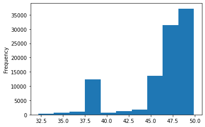
Now, with some simple histograms, we can have a visualization the distribution of each attribute in the dataset. This will allow us to look a little deeper than with the above functions.
For that, we use the method plot of a Pandas Series, which allows to produce different types of plot for an attribute, here we choose hist().
dynamic_data['LAT'].plot.hist()
<AxesSubplot:ylabel='Frequency'>

This plot shows the distribution of the latitude attribute in the dataset. We can see that many values are comprised in the range [45.0 ; 50.0]. This means that many positions are recorded in this area, while the range [32.5 ; 45.0] is less dense in recorded positions. If you want to know more about the histograms and the different kinds of plots used in the course, you can visit this page.
We can create this type of plot for every numerical attribute in the dataset.
In the previous cell, try to change the name of the plotted attribute to visualize the other attributes. You can even try to put the name of a non-numerical attribute to see what happens.
<function __main__.plot_hist(att)>
Finally, we can see the different values of each attribute.
For that, we use the method unique():
dynamic_data['VesselType'].unique()
array([  nan, 1012., 1019., 1001., 1025., 1024., 1004., 1018., 1005.,
         70.,   30., 1020.,   99., 1003.,   80., 1013.,   31., 1002.,
         52.,   53., 1011.,   50.,   35., 1023.,   69.,   37.,    7.,
         60., 1022.,   90.,   51., 1010.,    0.,   79.,   71., 1017.])
With this result, and by comparing the values with the AIS documention available here, you can analyze what kind of ships are present in the dataset.
Have a look at the different values for the other attributes by changing the name of the attribute in the previous cell.
<function __main__.get_unique(att)>
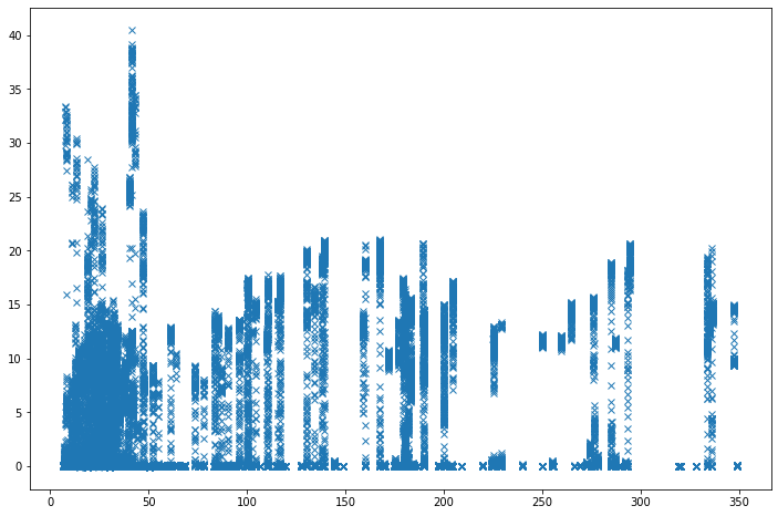
Additionaly, we can create a 2 dimensional plot, to represent 2 attributes against each other. For example, on this picture, we represent the attributes longitude and latitude, to get a geographical representation of the recorded datapoints:
import matplotlib.pyplot as plt

plt.figure(figsize = (12, 8))
plt.plot(dynamic_data['Length'], dynamic_data['SOG'], 'x')
[<matplotlib.lines.Line2D at 0x7f66d2f59cc0>]

The datapoints are represented as crosses, and on this plot, each separated blue line is a very likely one recorded trip.
Change the name of the attributes and try to compare other (numerical) attributes.
<function __main__.plot_2att(att1, att2)>
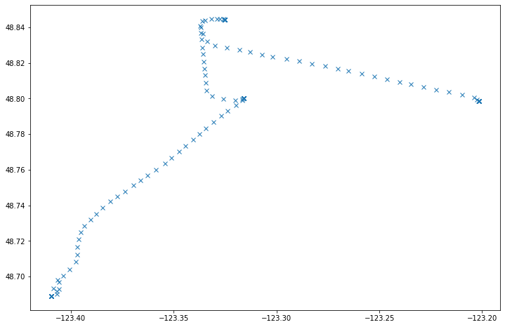
You can also choose to visualize the information of this dataset for only one trip. For example, we want to see the longitude and latitude values for the trip with the TripID 106:
# for one trip

trip = dynamic_data.loc[dynamic_data['TripID'] == 106]

plt.figure(figsize = (12, 8))
plt.plot(trip['LON'], trip['LAT'], 'x')
[<matplotlib.lines.Line2D at 0x7f66d1638668>]

Change the value of the TripID attribute, and the names of the attributes, to plot anything else.
<function __main__.plot_1trip(tripid, att1, att2)>
from IPython.display import IFrame
IFrame("https://h5p.org/h5p/embed/742748", "694", "600")
Static data - your turn 
Using the same tools as for the dynamic dataset, you can now analyze the static dataset.
static_data.info()
<class 'pandas.core.frame.DataFrame'>
RangeIndex: 1520 entries, 0 to 1519
Data columns (total 22 columns):
 #   Column      Non-Null Count  Dtype
---  ------      --------------  -----
 0   TripID      1520 non-null   int64
 1   MMSI        1520 non-null   int64
 2   MeanSOG     1520 non-null   float64
 3   VesselName  1442 non-null   object
 4   IMO         538 non-null    object
 5   CallSign    1137 non-null   object
 6   VesselType  1287 non-null   float64
 7   Length      1220 non-null   float64
 8   Width       911 non-null    float64
 9   Draft       496 non-null    float64
 10  Cargo       378 non-null    float64
 11  DepTime     1520 non-null   object
 12  ArrTime     1520 non-null   object
 13  DepLat      1520 non-null   float64
 14  DepLon      1520 non-null   float64
 15  ArrLat      1520 non-null   float64
 16  ArrLon      1520 non-null   float64
 17  DepCountry  1520 non-null   object
 18  DepCity     1520 non-null   object
 19  ArrCountry  1520 non-null   object
 20  ArrCity     1520 non-null   object
 21  Duration    1520 non-null   object
dtypes: float64(10), int64(2), object(10)
memory usage: 261.4+ KB
static_data.describe()
| TripID | MMSI | MeanSOG | VesselType | Length | Width | Draft | Cargo | DepLat | DepLon | ArrLat | ArrLon | |
|---|---|---|---|---|---|---|---|---|---|---|---|---|
| count | 1520.000000 | 1.520000e+03 | 1520.000000 | 1287.000000 | 1220.000000 | 911.000000 | 496.000000 | 378.000000 | 1520.000000 | 1520.000000 | 1520.000000 | 1520.000000 |
| mean | 760.500000 | 3.597421e+08 | 1.034825 | 971.680653 | 56.769590 | 13.104501 | 6.457056 | 50.515873 | 46.354331 | -122.868905 | 46.353671 | -122.871346 |
| std | 438.930518 | 6.263661e+07 | 2.936439 | 198.957887 | 74.739358 | 10.903338 | 4.607529 | 22.693810 | 3.766705 | 0.681947 | 3.762056 | 0.680604 |
| min | 1.000000 | 3.160089e+06 | -0.100000 | 0.000000 | 6.710000 | 0.000000 | 0.000000 | 0.000000 | 32.220640 | -125.995610 | 32.209370 | -125.998590 |
| 25% | 380.750000 | 3.380724e+08 | 0.000000 | 1004.000000 | 14.840000 | 5.500000 | 3.000000 | 31.000000 | 46.168653 | -123.178480 | 46.168460 | -123.168262 |
| 50% | 760.500000 | 3.669802e+08 | 0.012633 | 1019.000000 | 22.340000 | 8.000000 | 4.650000 | 52.000000 | 47.647795 | -122.651365 | 47.646925 | -122.645290 |
| 75% | 1140.250000 | 3.675663e+08 | 0.072000 | 1019.000000 | 41.277500 | 16.350000 | 10.025000 | 70.000000 | 48.656940 | -122.386562 | 48.665710 | -122.386607 |
| max | 1520.000000 | 9.876543e+08 | 20.360811 | 1025.000000 | 349.000000 | 50.000000 | 18.800000 | 99.000000 | 49.890740 | -120.002920 | 49.832120 | -120.002420 |
#static_data[''].plot.hist()
<function __main__.plot_hist(att)>
#static_data[''].unique()
<function __main__.get_unique(att)>
import matplotlib.pyplot as plt

plt.figure(figsize = (12, 8))
#plt.plot(static_data[''], static_data[''], 'x')
<Figure size 864x576 with 0 Axes>
<Figure size 864x576 with 0 Axes>
<function __main__.plot_2att(att1, att2)>
from IPython.display import IFrame
IFrame("https://h5p.org/h5p/embed/742791", "694", "600")

